Unsupervised ML with Penguins
Contents
Unsupervised ML with Penguins#
The palmer penguin dataset is excellent for EDA and UML. It contains different measures for 3 species of closely related penguins from several islands in Antarctica.
Let’s have a look:
Penguin datast: https://github.com/allisonhorst/palmerpenguins

# Install umap for dimensionality reduction
!pip install umap-learn -q
     |████████████████████████████████| 88 kB 4.2 MB/s
     |████████████████████████████████| 1.1 MB 16.5 MB/s
?25h  Building wheel for umap-learn (setup.py) ... ?25l?25hdone
  Building wheel for pynndescent (setup.py) ... ?25l?25hdone
# standard packaging

import pandas as pd
import seaborn as sns
sns.set(color_codes=True, rc={'figure.figsize':(10,8)})

from IPython.display import HTML #Youtube embed
In case you have a few minutes:
HTML('<iframe width="700" height="400" src="https://www.youtube-nocookie.com/embed/QS5jpQ6cpsg" frameborder="0" allow="accelerometer; autoplay; encrypted-media; gyroscope; picture-in-picture" allowfullscreen></iframe>')
/usr/local/lib/python3.7/dist-packages/IPython/core/display.py:701: UserWarning: Consider using IPython.display.IFrame instead
  warnings.warn("Consider using IPython.display.IFrame instead")
# load the dataset from GitHub - original source

penguins = pd.read_csv("https://github.com/allisonhorst/palmerpenguins/raw/5b5891f01b52ae26ad8cb9755ec93672f49328a8/data/penguins_size.csv")
# Check the data

penguins.head()
| species_short | island | culmen_length_mm | culmen_depth_mm | flipper_length_mm | body_mass_g | sex | |
|---|---|---|---|---|---|---|---|
| 0 | Adelie | Torgersen | 39.1 | 18.7 | 181.0 | 3750.0 | MALE |
| 1 | Adelie | Torgersen | 39.5 | 17.4 | 186.0 | 3800.0 | FEMALE |
| 2 | Adelie | Torgersen | 40.3 | 18.0 | 195.0 | 3250.0 | FEMALE |
| 3 | Adelie | Torgersen | NaN | NaN | NaN | NaN | NaN |
| 4 | Adelie | Torgersen | 36.7 | 19.3 | 193.0 | 3450.0 | FEMALE |
# drop all missing observations and count up the birds for each species

penguins = penguins.dropna()
penguins.species_short.value_counts()
Adelie       146
Gentoo       120
Chinstrap     68
Name: species_short, dtype: int64

# Let's check out the data visually

sns.pairplot(penguins, hue='species_short', kind="reg", corner=True, markers=["o", "s", "D"], plot_kws={'line_kws':{'color':'white'}})
<seaborn.axisgrid.PairGrid at 0x7fae91b3ce90>
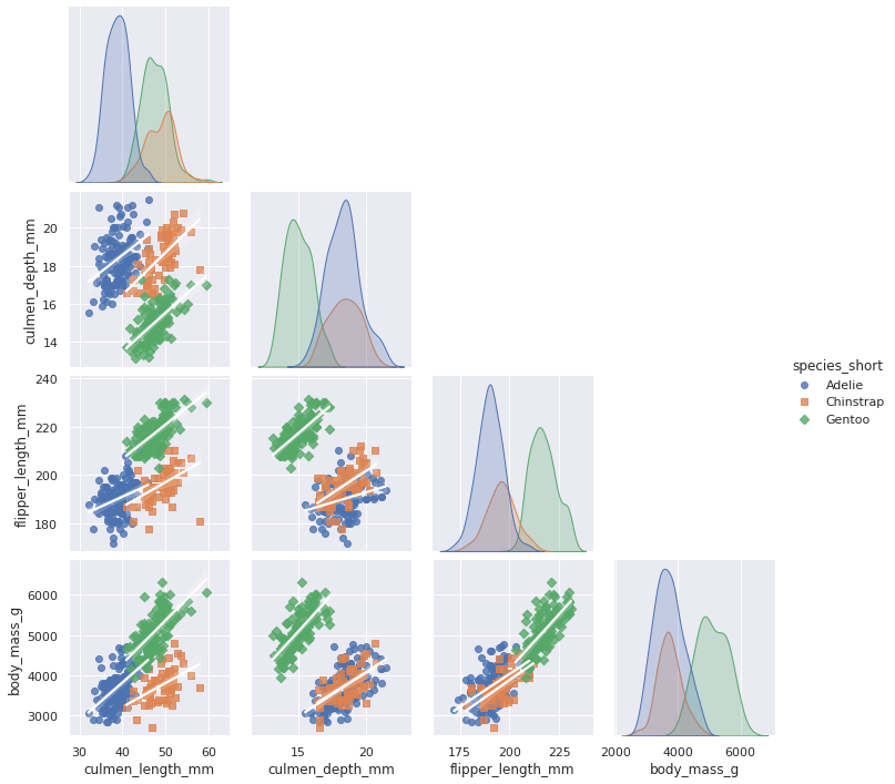
Overall we can see some general tendencies in the data:
Being “bio” data, it is rather normally distributed
Gentoos are on average heavier
Glipper length is correlated with body mass for all species
Culmen length and depth is correlated with body mass for gentoos but not so much for the other species (visual analysis…no proper calculation)
Overall there is obviousely some correlation between the variables that can be ‘exploited’ for dimensionality reduction.
Before we can do any machine learning, it is a good idea to scale the data. Most algorithms are not agnostic to magnitudes and bringing all variables on the same scale is therefore crucial.
# We load up Standard Scaler from sklearn

from sklearn.preprocessing import StandardScaler
# And scale all relevant variables into a new matrix (numpy)

scaled_penguins = StandardScaler().fit_transform(penguins.loc[:,'culmen_length_mm':'body_mass_g'])
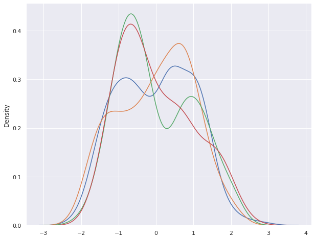
# all variables now have a mean of 0 and std of 1
for i in range(4):
  sns.distplot(scaled_penguins[:,i], hist=False)
/usr/local/lib/python3.7/dist-packages/seaborn/distributions.py:2619: FutureWarning: `distplot` is a deprecated function and will be removed in a future version. Please adapt your code to use either `displot` (a figure-level function with similar flexibility) or `kdeplot` (an axes-level function for kernel density plots).
  warnings.warn(msg, FutureWarning)
Econometrics detour#
Python is not known for that but Statsmodels has in the past few years become a decent package for econometrics. Let’s see if we can quickly put a model to estimate the relationship most variables and DV culmen lenght.
import statsmodels.api as sm
from patsy import dmatrices
y, X = dmatrices('culmen_length_mm ~ culmen_depth_mm + flipper_length_mm + body_mass_g', data=penguins, return_type='dataframe')
X.head()
| Intercept | culmen_depth_mm | flipper_length_mm | body_mass_g | |
|---|---|---|---|---|
| 0 | 1.0 | 18.7 | 181.0 | 3750.0 |
| 1 | 1.0 | 17.4 | 186.0 | 3800.0 |
| 2 | 1.0 | 18.0 | 195.0 | 3250.0 |
| 4 | 1.0 | 19.3 | 193.0 | 3450.0 |
| 5 | 1.0 | 20.6 | 190.0 | 3650.0 |
mod = sm.OLS(y, X) # Describe model
res = mod.fit() # Fit model
print(res.summary()) # Summarize model
                            OLS Regression Results
==============================================================================
Dep. Variable:       culmen_length_mm   R-squared:                       0.459
Model:                            OLS   Adj. R-squared:                  0.454
Method:                 Least Squares   F-statistic:                     93.40
Date:                Sat, 20 Aug 2022   Prob (F-statistic):           8.84e-44
Time:                        13:16:19   Log-Likelihood:                -937.75
No. Observations:                 334   AIC:                             1884.
Df Residuals:                     330   BIC:                             1899.
Df Model:                           3
Covariance Type:            nonrobust
=====================================================================================
                        coef    std err          t      P>|t|      [0.025      0.975]
-------------------------------------------------------------------------------------
Intercept           -25.5118      6.709     -3.803      0.000     -38.709     -12.314
culmen_depth_mm       0.6136      0.138      4.440      0.000       0.342       0.885
flipper_length_mm     0.2859      0.035      8.155      0.000       0.217       0.355
body_mass_g           0.0004      0.001      0.630      0.529      -0.001       0.001
==============================================================================
Omnibus:                       27.525   Durbin-Watson:                   0.880
Prob(Omnibus):                  0.000   Jarque-Bera (JB):               36.609
Skew:                           0.610   Prob(JB):                     1.12e-08
Kurtosis:                       4.070   Cond. No.                     1.30e+05
==============================================================================

Notes:
[1] Standard Errors assume that the covariance matrix of the errors is correctly specified.
[2] The condition number is large, 1.3e+05. This might indicate that there are
strong multicollinearity or other numerical problems.
Back to UML, dimensionality reduction and clustering#
# Let's import PCA
from sklearn.decomposition import PCA
pca = PCA(n_components=2) # we explicitly ask for 2 components
# And now we use PCA to transform the data
pca_penguins = pca.fit_transform(scaled_penguins)
pca_penguins.shape # 334 rows, 2 columns - just as we wanted
(334, 2)
The two components should now contains information that describes the data but where the information within the two should be maximally dissimilar. Since we now have 2 dimension describing each observation, we can plot them against each other in a scatterplot.
You want to learn more about PCA and the math behind it? Check out the chapter in the book: https://jakevdp.github.io/PythonDataScienceHandbook/05.09-principal-component-analysis.html
sns.scatterplot(pca_penguins[:,0], pca_penguins[:,1], hue = penguins['species_short'] )

# note that we are using numpy-indexing [:,0] means: all rows and only first column!!!

# we use the colors of the species that we know to see how well the PCA did...
/usr/local/lib/python3.7/dist-packages/seaborn/_decorators.py:43: FutureWarning: Pass the following variables as keyword args: x, y. From version 0.12, the only valid positional argument will be `data`, and passing other arguments without an explicit keyword will result in an error or misinterpretation.
  FutureWarning
<matplotlib.axes._subplots.AxesSubplot at 0x7fae8c747bd0>
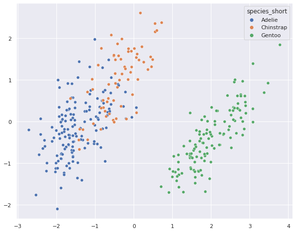
Not too bad. We colo Now let’s try out UMAP, a new dimensionality reduction algorightm that comes with many interesting features: https://umap-learn.readthedocs.io/en/latest/
You want to learn more from the guy behind the algorithm? https://youtu.be/nq6iPZVUxZU check out that excellent talk by Leland McInnes or https://arxiv.org/abs/1802.03426.
# Let's load umap and instantiate it 2-components is standard and we don't need to specify it

import umap
reducer = umap.UMAP()
# let's reduce the scalded data - same syntax as sklearn :-)

umap_penguins = reducer.fit_transform(scaled_penguins)
umap_penguins.shape
(334, 2)
# Let's plot the matrix

sns.scatterplot(umap_penguins[:,0], umap_penguins[:,1], hue = penguins['species_short'] )
/usr/local/lib/python3.7/dist-packages/seaborn/_decorators.py:43: FutureWarning: Pass the following variables as keyword args: x, y. From version 0.12, the only valid positional argument will be `data`, and passing other arguments without an explicit keyword will result in an error or misinterpretation.
  FutureWarning
<matplotlib.axes._subplots.AxesSubplot at 0x7fae22e6db90>
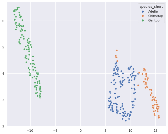
Umap seems to do a better job at reducing the dimensionality in a way that the resulting embedding fits well with the species destinction.
Clustering#
Now that we had a look at dimensionality reduction, let’s see what clustering can do at the present case.
We will try out K-means and hierarchical clustering
# we import kmeans
from sklearn.cluster import KMeans
# and instantiate it where we need to specify that we want it to create 3 clusters

clusterer = KMeans(n_clusters=3)
clusterer.fit(scaled_penguins) #we only fit here, since no data needs to be transformed
KMeans(n_clusters=3)
# now let's see how well the clusters fit with the species

sns.scatterplot(umap_penguins[:,0], umap_penguins[:,1], hue = clusterer.labels_ )
/usr/local/lib/python3.7/dist-packages/seaborn/_decorators.py:43: FutureWarning: Pass the following variables as keyword args: x, y. From version 0.12, the only valid positional argument will be `data`, and passing other arguments without an explicit keyword will result in an error or misinterpretation.
  FutureWarning
<matplotlib.axes._subplots.AxesSubplot at 0x7fae21b0b3d0>
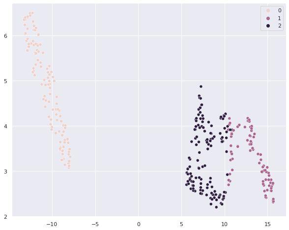
# we can check out a cross-tab with clusters vs. species
pd.crosstab(clusterer.labels_, penguins['species_short'])
| species_short | Adelie | Chinstrap | Gentoo |
|---|---|---|---|
| row_0 | |||
| 0 | 0 | 0 | 120 |
| 1 | 22 | 63 | 0 |
| 2 | 124 | 5 | 0 |
Now let’s turn to hierarchical clustering - the procedure is the same, we just need to swap the algorithm name
from sklearn.cluster import AgglomerativeClustering
clusterer = AgglomerativeClustering(n_clusters=3).fit(scaled_penguins)
sns.scatterplot(umap_penguins[:,0], umap_penguins[:,1], hue = clusterer.labels_ )
/usr/local/lib/python3.7/dist-packages/seaborn/_decorators.py:43: FutureWarning: Pass the following variables as keyword args: x, y. From version 0.12, the only valid positional argument will be `data`, and passing other arguments without an explicit keyword will result in an error or misinterpretation.
  FutureWarning
<matplotlib.axes._subplots.AxesSubplot at 0x7fae21a47250>
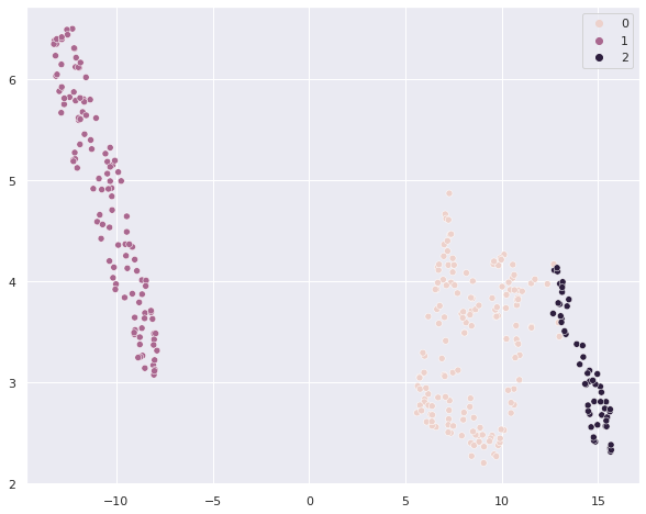
# Let's do the cross-tab with clusters vs. species
pd.crosstab(clusterer.labels_, penguins['species_short'])
| species_short | Adelie | Chinstrap | Gentoo |
|---|---|---|---|
| row_0 | |||
| 0 | 146 | 11 | 0 |
| 1 | 0 | 0 | 120 |
| 2 | 0 | 57 | 0 |